NPV in Excel

This pages teach you how to calculate the Net Present Value (NPV) of an investment project, using Microsoft Excel.

To calculate the NPV you will need the initial investment and all the future cash flows. Usually, the NPV is used to analyze the profitability of an investment that will happen in the future. This is why all the future cash flows are usually estimations or projections.

In the NPV, the Discount Rate should be the highest rate of return available to invest, with a similar risk to the current investment project. The discount rate is very important in the calculation of the NPV, but at the same time, it can be very difficult to estimate, because it's usually very difficult to estimate the risk of an investment project.

If the project is financed using external capital, companies can chose the Weighted Average Cost of Capital (WACC) as a discount rate.

Select a cell (e.g. A2) ant type “Year”. Below the cell, insert 1,2,3… in each cell. For example, if your investment project lasts 5 years, you will end with a column like the following:

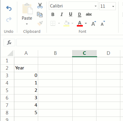
Note the number “0”. It's because the initial investment is done in the year “0”.

If you have the data by months, you have to put the months in the first column. But take into account that the discount rate must be a monthly rate.

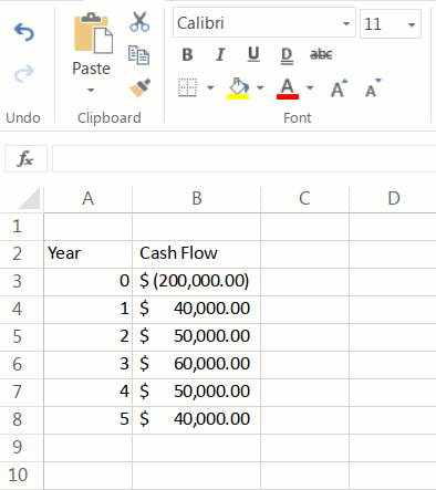
In the second column, you will input the cash flow corresponding to each year. For the “0” year, insert the initial investment.

A project can have many years with a negative cash flow. The calculation doesn't change.

If you plan to sell the business in the future, in the last year the cash flow must include the inflow of funds resulting from the sale.

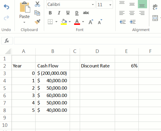
Select a cell and insert “Discount Rate”. In the cell below or next, insert the discount rate. For example, if the discount rate is 6%, type “0.06”.

Click in a cell in which you want to calculate the NPV and:

1. type “=NPV(”
2. select the cell where you typed the discount rate (“E2” in our example)
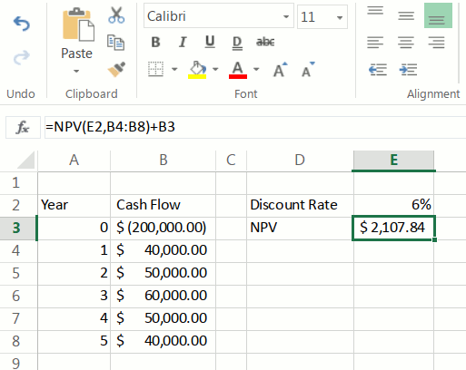
3. select the cell range that contains the future cash flows (“C5:C9” in our example). Do not select the initial investment.
4. close the formula, insert “)”. If you press enter, you will have the present value of all future cash flows at period zero.
5. add the initial investment: at the end of the previous formula, in the same cell, insert “+” and select the cell containing the initial investment. (B3 in our example). Press enter and you will have calculated the NPV in Excel.

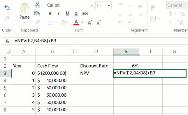
The final formula looks like this:

=NPV(E2,B4:B8)+B3

Actually, the Excel NPV formula does not calculate the Net Present Value, but the value of a series of cash flows at period zero. That is why we enter only the future cash flows in the formula and then subtract the initial investment, that is, the cash flow at period zero.

If someone includes the initial investment in the NPV formula, it's wrong.